Two Variable Data Table In Excel – Easy 4 Step Guide

In part 01 of this tutorial you learned the basics of Microsoft excel data tables and how to use one variable data table.
It is more useful if we can evaluate formulas against the change of values of two variables instead of one variable.

We can use Microsoft Excel two variable Data Tables to evaluate the results of a calculation formula for different combination of values for two variables.

Even though we can evaluate multiple calculations simultaneously using the one variable data table, we can only evaluate a single calculation formula here. But you may find it is very useful in some situations.

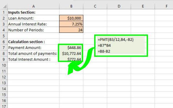
As an example we can use a two variable data table to evaluate & and analysis different loan schemes having different interest rates for different loan duration. We can use this feature to review the compare the loan payment amount due for a period, total amount of payments or the total amount of the interest portion of the loan payments.

Steps to setup and use two variable Data Tables

Step 01: Prepare the input section and calculation section

You could easily follow the same steps as you did during the part 01. Click here if you missed that tutorial.

Step 02: Prepare the Two Variable Data table section

Prepare your excel worksheet as shown in the below figure. You could see that there is a difference of the layout of the table when you compare it to the single variable data table. In two variable data-table, you put your values for one variable along the cells of column header and the values for the second variable should be inserted in the row header cells located along the left edge of the table range.

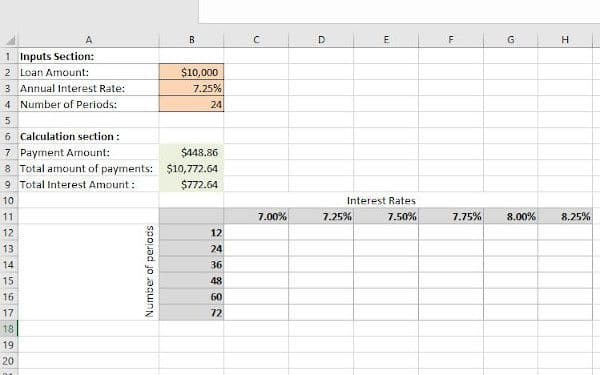
In this example we are going to see what will be the result of selected loan calculation formula if we change the annual interest rate & total number payment periods.

So we will enter our different interest rates within the cells in the range C11:H11 and the total number of payment periods (Months in this example) are will be entered within the cells of the range B12:B17

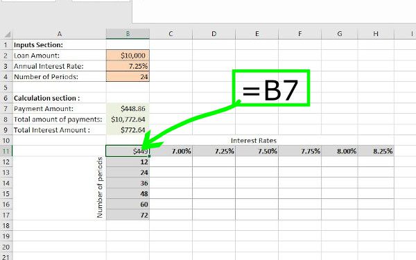
Step 03: Insert or link the calculation formula to the Data-Table

Now insert the relevant cell reference formula for the selected loan calculation formula within the top-left corner cell of Data-Table cell range. Remember that you will be able only to evaluate the results set of one loan calculation formula at a time. Therefore, you would need to change the cell reference formula inserted within the top-left corner cell as and when required.

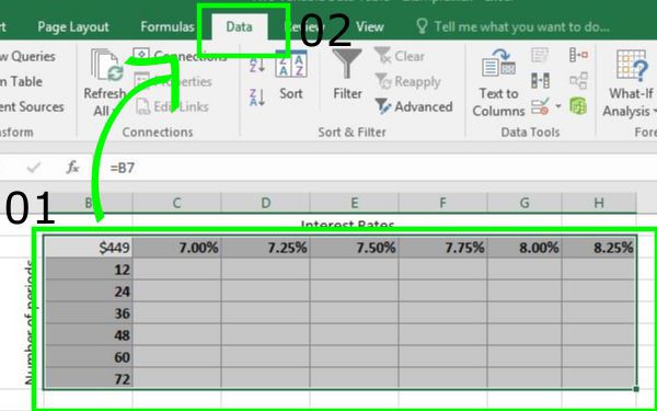
Step 04: Select the Data Table cell range and Invoke Microsoft excel Data Table tool

Select cell range that has the Data-Table, then Go to “Data” Tab

Then,

Go to “Data Analysis” Command group → Click “What-If-Analysis” → Select “Data Tables” from the appeared drop down menu.

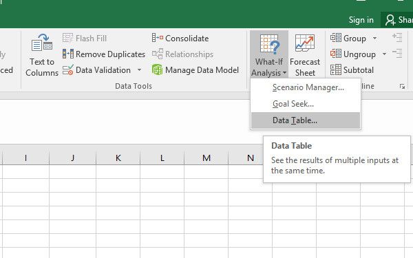
Now, the “Data Table” dialog box appears.

Place the cursor inside the “Row input cell” input box and select the cell B3 where the input value for annual interest rate is entered.
Then, place the cursor inside the “Column input cell” input box and select the cell B4 where the input value for total number of payment periods is entered.

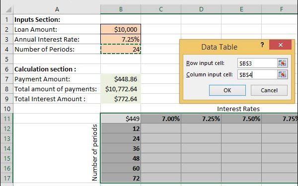
Click “OK“.

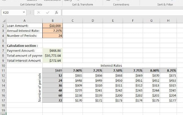
It will generate the results for the selected calculation formula based on the different input value combinations for the total number of payment periods and the annual interest rate.

Interpretation of the results

You got the results for the selected calculation formula with respect to each possible interest rate and loan period combination.

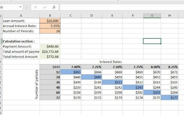
But in real world situations you would not get offered this all kinds of loan schemes. You get lower interest rate for short-duration loan and get higher interest rate for long-duration loan.

Therefore, most probably you get only one interest rate for given number of loan periods. If that is the case, you can easily highlight the cells that return the output for the relevant interest rate and payment periods combinations. And then pay attention to the highlighted cells to compare cost and benefits of each loan scheme.

Download this example excel file for two variable Data Table.

This tutorial created using Microsoft Excel 2016. Other compatible versions are Excel for Office 365 Excel for Office 365 for Mac; Excel 2016; Excel 2019 for Mac; Excel 2013; Excel 2010; Excel 2007; Excel 2016 for Mac; Excel for Mac 2011. If you find any issues doing regression analysis in those versions, please leave a comment below.